When dealing with classification problems in Machine Learning, one of the things we have to take into account is the balance of the classes that define the label.
Imagine a scenario where we have a three-class problem. We make our initial analyses, calculate accuracy, and get 93%. Then, we go deeper and see that 80% of the data belongs to one class. Is that a good sign?
Well, it’s not, and this article will explain why.
For Newcomers: Getting Setup with Jupyter Notebooks
If you’re a beginner in Machine Learning, you may not know that to handle an ML problem you can use two software:
Anaconda is a Data Science platform that provides you with all the libraries you’ll need to analyze data and make predictions with machine learning. It also provides you with Jupyter Notebooks that are the environment data scientists use to analyze data. So, once you install Anaconda, you have everything you need.
Google Colaboratory, instead, is a hosted Jupyter Notebook service that requires no setup to use and provides free access to computing resources as well as all the libraries you need. So, if you don’t want to install anything on your PC, you can choose this solution for analyzing your data.
Finally, I created a public repository that hosts all the code you’ll find in this article in a unique Jupyter Notebook, so that you can consult it and see how data scientists structure Jupyter Notebooks to analyze data.
Introduction to Imbalanced Data in Machine Learning
This section introduces the problem of class imbalance in Machine Learning and covers scenarios where imbalanced classes are common. But before going on, let’s say that we can use the terms “unbalanced” or “imbalanced” indifferently.
Defining Imbalanced Data and its Implications on Model Performance
Imagine you’re the math teacher of a group of 100 students. Now, among these students, 90 are good at math (let’s call them Group A), while 10 struggle with it (Group B). This class makeup represents what we call “imbalanced data” in the world of machine learning.
In Machine Learning, data is like the textbook you use to teach a computer to make predictions or decisions. When you have imbalanced data, it means that there’s a big difference in the number of examples for different things the computer is supposed to learn. In our classroom analogy, there’s a huge number of students in Group A (the majority class) compared to the small number of students in Group B (the minority class).
Now, the performance of our ML models is affected by imbalanced data. For example, these are the implications:
- Biased Learning. If you teach your computer using this imbalanced classroom, where most students are good at math, it might get a bit biased. It’s like the computer is surrounded by excellent math students all the time, so it might think that everyone is a math genius. In machine learning terms, the model can become biased towards the majority class. It becomes good at predicting what’s common (Group A) but struggles to understand the less common stuff (Group B). In other words, if you’re evaluating how good are you at teaching math by using the votes of your students, you’ll get a biased result because 90% of your students are good at math. But how about the majority of this 90% are taking private lessons and you don’t know?
- Misleading Accuracy. Imagine you evaluate the computer’s performance by checking how many students it correctly identifies as good or struggling in math. Since there are so many in Group A, the computer could get most of them right. So, it looks like the computer is doing a fantastic job because its “accuracy” is high. However, it’s actually failing miserably with Group B because there are so few students in that group. In Machine Learning, this high accuracy can be misleading because it doesn’t tell you how well the computer is doing in the minority class.
In a nutshell, imbalanced data means you have an unequal number of examples for different things you want your computer to learn, and it can seriously affect how well your Machine Learning model works, especially when it comes to handling the less common cases.
Anyway, there are cases where we expect the data to be unbalanced.
Let’s see some of them before describing how we can deal with them.
Scenarios Where Imbalanced Data is Common
In real-life scenarios, there are situations where we expect the data to be unbalanced. And, if they’re not, it means that there are some errors.
For example, let’s consider the medical field. If we’re trying to find a rare disease in a big population, the data has to be unbalanced, otherwise the disease we’re searching for is not rare.
Similarly, in fraud detection. If we’re a Data Scientist in a finance firm and are analyzing fraudulent transactions on credit cards, the obvious expectation is that we find imbalanced data. Otherwise, this means that fraudulent transactions occur as many times as non-fraudulent transactions.
Understanding the Imbalance Problem
Now, let’s dive into a practical situation with some Python code so that we can show:
- The difference between the majority and minority classes on a graphical base.
- The evaluation metrics affected by imbalanced data.
- The evaluation metrics not affected by imbalanced data.
Difference Between Majority and Minority Classes
Suppose you’re still a math teacher, but this time in a greater class with 1000 students. Before making any classification with Machine Learning, you decide to verify if the data you have is imbalanced or not.
One method we can use is by visualizing the distribution. For example, like so:
import numpy as np
import matplotlib.pyplot as plt

# Set random seed for reproducibility
np.random.seed(42)

# Generate data for a majority class (Class 0)
majority_class = np.random.normal(0, 1, 900)

# Generate data for a minority class (Class 1)
minority_class = np.random.normal(3, 1, 100)

# Combine the majority and minority class data
data = np.concatenate((majority_class, minority_class))

# Create labels for the classes
labels = np.concatenate((np.zeros(900), np.ones(100)))

# Plot the class distribution
plt.figure(figsize=(8, 6))
plt.hist(data[labels == 0], bins=20, color='blue', alpha=0.6, label='Majority Class (Class 0)')
plt.hist(data[labels == 1], bins=20, color='red', alpha=0.6, label='Minority Class (Class 1)')
plt.xlabel('Feature Value')
plt.ylabel('Frequency')
plt.title('Class Distribution in an Imbalanced Dataset')
plt.legend()
plt.show()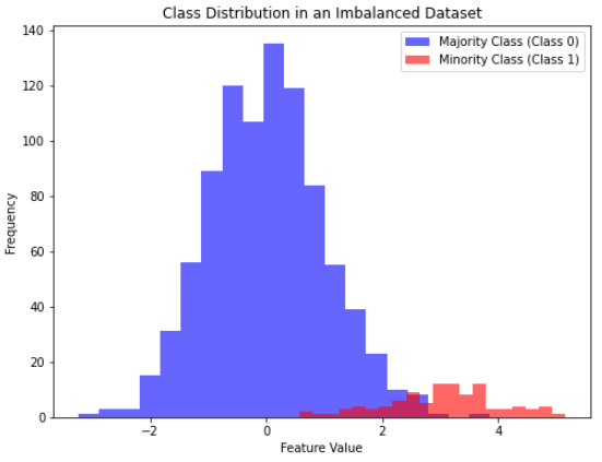
In this Python example, we’ve created two classes:
- Majority Class (Class 0). This class represents the majority of the data points. We generated 900 data points from a normal distribution with a mean of 0 and a standard deviation of 1. In a real-world scenario, this could represent something very common or typical.
- Minority Class (Class 1). This class represents the minority of the data points. We generated 100 data points from a normal distribution with a mean of 3 and a standard deviation of 1. This class is intentionally made less common to simulate an imbalanced dataset. In practice, this could represent rare events or anomalies.
Next, we combine these two classes into a single dataset with corresponding labels (0 for the majority class and 1 for the minority class). Finally, we visualize the class distribution using a histogram. In the histogram:
- The blue bars represent the majority class (Class 0), which is the taller and more frequent bar on the left side.
- The red bars represent the minority class (Class 1), which is the shorter and less frequent bar on the right side.
This visualization clearly shows the difference between the majority and minority classes in an imbalanced dataset. The majority class has many more data points than the minority class, which is a common characteristic of imbalanced data.
Another way to look at class imbalance is to directly look at the frequencies, without going through the distributions, if we prefer. For example, we can do it like so:
import numpy as np
import matplotlib.pyplot as plt

# Set a random seed for reproducibility
np.random.seed(42)

# Generate data for a majority class (Class 0)
majority_class = np.random.normal(0, 1, 900)

# Generate data for a minority class (Class 1)
minority_class = np.random.normal(3, 1, 100)

# Combine the majority and minority class data
data = np.concatenate((majority_class, minority_class))

# Create labels for the classes
labels = np.concatenate((np.zeros(900), np.ones(100)))

# Count the frequencies of each class
class_counts = [len(labels[labels == 0]), len(labels[labels == 1])]

# Plot the class frequencies using a bar chart
plt.figure(figsize=(8, 6))
plt.bar(['Majority Class (Class 0)', 'Minority Class (Class 1)'], class_counts, color=['blue', 'red'])
plt.xlabel('Classes')
plt.ylabel('Frequency')
plt.title('Class Frequencies in an Imbalanced Dataset')
plt.show()
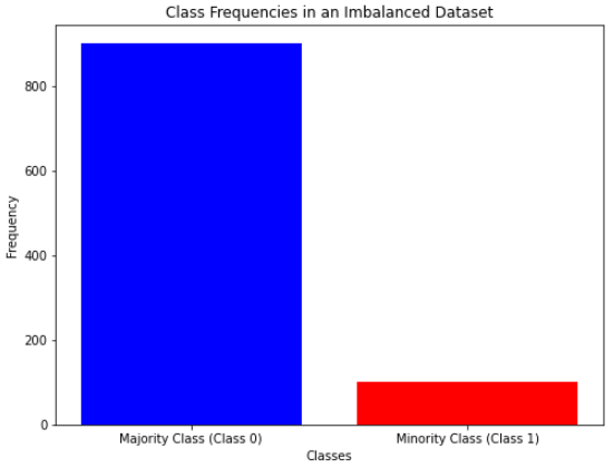
So, in this case, we can use the built-in method len() to calculate all the occurrences of the data belonging to a class.
Common Evaluation Metrics That Are Affected by Imbalanced Data
To describe all the metrics that are affected by imbalanced data we first have to define the following:
- True positive (TP). A correctly predicted value by a classifier indicating the presence of a condition or characteristic
- True negative (TN). A correctly predicted value by a classifier indicating the absence of a condition or characteristic
- False positive (FP). A wrongly predicted value by a classifier indicating that a particular condition or attribute is present when it’s not.
- False negative (FN). A wrongly predicted value by a classifier indicates that a particular condition or attribute is not present when it is.
Here are the common evaluation metrics affected by imbalanced data:
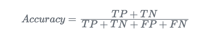
- Accuracy. It measures the ratio of correctly predicted instances to the total instances in the dataset:
Let’s make a Python example of how to calculate the accuracy metric:
from sklearn.metrics import accuracy_score

# True labels

true_labels = [0, 0, 0, 0, 0, 1, 1, 1, 1, 1]

# Predicted labels by a model
predicted_labels = [0, 0, 0, 0, 0, 0, 0, 0, 0, 0]

accuracy = accuracy_score(true_labels, predicted_labels)
print("Accuracy:", accuracy)
The result is:
Accuracy: 0.5
Accuracy can be misleading when dealing with imbalanced data.
In fact, suppose we have a dataset with 95% of instances belonging to Class A and only 5% to Class B. If a model predicts all instances as Class A, it would achieve an accuracy of 95%. However, this doesn’t necessarily mean the model is good; it’s just exploiting the class imbalance. This metric, in other words, doesn’t account for how well the model identifies the minority class (Class B).
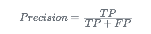
- Precision. It measures the proportion of correctly predicted positive instances out of all predicted positive instances:
Let’s make a Python example of how to calculate the precision metric:
from sklearn.metrics import precision_score

# True labels
true_labels = [0, 0, 0, 0, 0, 1, 1, 1, 1, 1]

# Predicted labels by a model
predicted_labels = [1, 1, 1, 1, 1, 1, 1, 1, 1, 1]

precision = precision_score(true_labels, predicted_labels)
print("Precision:", precision)
The result is:
Precision: 0.5
In imbalanced datasets, precision can be highly misleading.
In fact, if a model classifies only one instance as positive (Class B) and it’s correct, the precision would be 100%. However, this doesn’t indicate the model’s performance on the minority class because it may be missing many positive instances.
- Recall (or sensitivity). Recall, also known as sensitivity or true positive rate, measures the proportion of correctly predicted positive instances out of all actual positive instances:
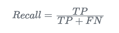
Let’s make a Python example of how to calculate the recall metric:
from sklearn.metrics import recall_score

# True labels
true_labels = [0, 0, 0, 0, 0, 1, 1, 1, 1, 1]

# Predicted labels by a model
predicted_labels = [1, 1, 1, 1, 1, 1, 1, 1, 1, 1]

recall = recall_score(true_labels, predicted_labels)
print("Recall:", recall)
The result is:
Recall: 1.0
Recall can also be misleading in imbalanced datasets, especially when it’s crucial to capture all positive instances.
If a model predicts only one instance as positive (Class B) when there are more positive instances, the recall may be very low, indicating that the model is missing a significant portion of the minority class. This happens because this metric doesn’t consider false positives.
- F1 score. The F1-score is the harmonic mean of precision and recall. It provides a balance between precision and recall:
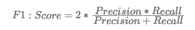
Let’s make a Python example of how to calculate the F1 score metric:
from sklearn.metrics import f1_score

# True labels
true_labels = [0, 0, 0, 0, 0, 1, 1, 1, 1, 1]

# Predicted labels by a model
predicted_labels = [1, 1, 1, 1, 1, 1, 1, 1, 1, 1]

# Calculate and print F1-score
f1 = f1_score(true_labels, predicted_labels)
print("F1-Score:", f1)
The result is:
F1-Score: 0.6666666666666666
As this metric is created using precision and recall, it can be affected by imbalanced data.
If one class is heavily dominant (the majority class), and the model is biased towards it, the F1-score may still be relatively high due to high precision but low recall for the minority class. This could misrepresent the model’s overall effectiveness.
Most Used Evaluation Metrics That Are Not Affected by Imbalanced Data
Now we’ll describe the two most used evaluation metrics among all of those that are not affected by class imbalance.
- Confusion matrix. A confusion matrix is a table that summarizes the performance of a classification algorithm. It provides a detailed breakdown of true positives (TP), true negatives (TN), false positives (FP), and false negatives (FN). In particular, the primary diagonal (upper-left to lower-right) shows the TPs and TN. The secondary diagonal (lower-left to upper-right) shows us FP and FN. So, if an ML model is correctly classifying the data, the primary diagonal of the confusion matrix should report the highest values, while the secondary is the lowest.
Let’s show an example in Python:
from sklearn.metrics import confusion_matrix

# True and predicted labels
true_labels = [0, 0, 0, 0, 0, 1, 1, 1, 1, 1]
predicted_labels = [0, 0, 0, 0, 0, 1, 1, 1, 0, 1]

# Create confusion mateix
cm = confusion_matrix(true_labels, predicted_labels)

# Print confusion matrix
print("Confusion Matrix:")
print(cm)
And we get:
Confusion Matrix:
[[5 0]
 [1 4]]
So, this confusion matrix represents a good classifier because the primary diagonal has the most results (9 out of 10). This means that the classifier predicts 5 TPs and 4 TNs.
The secondary diagonal, instead, has the lower results (1 out of 10). This means that the classifier has predicted one FP and 0 FNs.
Thus, this results in a good classifier.
So, the confusion matrix provides a detailed breakdown of model performance, making it easy to see how many instances are correctly or incorrectly classified for each class in a matter of seconds.
- AUC/ROC curve. ROC stands for “Receiver Operating Characteristic” and is a graphical way to evaluate a classifier by plotting the true positive rate (TPR) against the false positive rate (FPR) at different thresholds.
We define:
- TPR as the sensitivity (which can also be called recall, as we said).
- FPR as 1-specificity.
Specificity is the ability of a classifier to find all the negative samples:
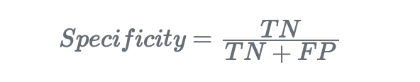
AUC, instead, stands for “Area Under Curve” and represents the area under the ROC curve. So this is an overall performance method, ranging from 0 to 1 (where 1 means the classifier predicts 100% of the labels as the actual values), and it’s more suitable when comparing different classifiers.
Suppose we’re studying a binary classification problem. This is how we can plot an AUC curve in Python:
import numpy as np
from sklearn.datasets import make_classification
from sklearn.model_selection import train_test_split
from sklearn.linear_model import LogisticRegression
from sklearn.metrics import roc_curve, roc_auc_score
import matplotlib.pyplot as plt

# Generate a random binary classification dataset
X, y = make_classification(n_samples=1000, n_features=10, n_classes=2,
       random_state=42)

# Split the dataset into training and testing sets
X_train, X_test, y_train, y_test = train_test_split(X, y,
                                  test_size=0.2, random_state=42)

# Fit a logistic regression model on the training data
model = LogisticRegression()
model.fit(X_train, y_train)

# Predict probabilities for the testing data
probs = model.predict_proba(X_test)

# Compute the ROC curve and AUC score
fpr, tpr, thresholds = roc_curve(y_test, probs[:, 1])
auc_score = roc_auc_score(y_test, probs[:, 1])

# Plot the ROC curve
plt.plot(fpr, tpr, label='AUC = {:.2f}'.format(auc_score))
plt.plot([0, 1], [0, 1], 'k--')
plt.xlabel('False Positive Rate')
plt.ylabel('True Positive Rate')
plt.title('ROC Curve')
plt.legend(loc='lower right')
plt.show()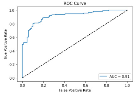
So, with this code, we have:
- Generated a classification dataset with the method
make_classification. - Splitted the dataset into the train and test sets.
- Fitted the train set with a Logistic Regression classifier.
- Made predictions on the test with the method
predict_proba() - Computed the ROC curve and AUC score.
- Plotted the AUC curve.
Techniques to Handle Imbalanced Data
In this section, we’ll cover some techniques to handle imbalanced data.
In other words: we’ll discuss how to manage imbalanced data when they shouldn’t.
Resampling
A widely adopted methodology for dealing with unbalanced datasets is resampling. This methodology can be separated into two different processes:
- Oversampling. It consists in adding more examples to the minority class.
- Undersampling. It consists in removing samples from the majority class.
Let’s explain them both.
Oversampling
Oversampling is a resampling technique that aims to balance the class distribution by increasing the number of instances in the minority class. This is typically done by either duplicating existing instances or generating synthetic data points similar to the minority class. The goal is to ensure that the model sees a more balanced representation of both classes during training.
Pros:
- Improved model performance. Oversampling helps the model better learn the characteristics of the minority class, leading to improved classification performance, especially for the minority class.
- Preserves information. Unlike undersampling, oversampling retains all instances from the majority class, ensuring that no information is lost during the process.
Cons:
- Overfitting risk. Duplicating or generating synthetic instances can lead to overfitting if not controlled properly, especially if the synthetic data is too similar to the existing data.
- Increased training time. A larger dataset due to oversampling may result in longer training times for machine learning algorithms.
Here’s how we can use the oversampling technique in Python on an imbalanced dataset:
import numpy as np
import matplotlib.pyplot as plt
from sklearn.datasets import make_classification
from imblearn.over_sampling import RandomOverSampler
from collections import Counter

# Create an imbalanced dataset with 3 classes
X, y = make_classification(
    n_samples=1000,
    n_features=20,
    n_classes=3,
    n_clusters_per_class=1,
    weights=[0.1, 0.3, 0.6],  # Class imbalance
    random_state=42
)

# Print the histogram of the initial classes
plt.figure(figsize=(10, 6))
plt.hist(y, bins=range(4), align='left', rwidth=0.8, color='blue', alpha=0.7)
plt.title("Histogram of Initial Classes")
plt.xlabel("Class")
plt.ylabel("Number of Instances")
plt.xticks(range(3), ['Class 0', 'Class 1', 'Class 2'])
plt.show()

# Apply oversampling using RandomOverSampler
oversampler = RandomOverSampler(sampling_strategy='auto', random_state=42)
X_resampled, y_resampled = oversampler.fit_resample(X, y)

# Print the histogram of the resampled classes
plt.figure(figsize=(10, 6))
plt.hist(y_resampled, bins=range(4), align='left', rwidth=0.8, color='orange', alpha=0.7)
plt.title("Histogram of Resampled Classes (Oversampling)")
plt.xlabel("Class")
plt.ylabel("Number of Instances")
plt.xticks(range(3), ['Class 0', 'Class 1', 'Class 2'])
plt.show()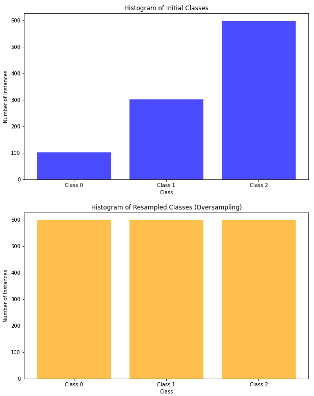
Undersampling
Undersampling is a resampling technique in machine learning that focuses on balancing the class distribution by reducing the number of instances in the majority class. This is typically achieved by randomly removing instances from the majority class until a more balanced representation of both classes is achieved. Here are the pros and cons of undersampling.
Pros:
- Reduced overfitting risk. Undersampling reduces the risk of overfitting compared to oversampling. By decreasing the number of instances in the majority class, the model is less likely to memorize the training data and can generalize better to new, unseen data.
- Faster training time. With fewer instances in the dataset after undersampling, the training time for machine learning algorithms may be reduced. Smaller datasets generally result in faster training times.
Cons:
- Loss of information. Undersampling involves discarding instances from the majority class, potentially leading to a loss of valuable information. This can be problematic if the discarded instances contain important characteristics that contribute to the overall understanding of the majority class.
- Risk of biased model. Removing instances from the majority class may lead to a biased model, as it might not accurately capture the true distribution of the majority class. This bias can affect the model’s ability to generalize to real-world scenarios.
- Potential Poor Performance on Majority Class. Undersampling may lead to a model that performs poorly on the majority class since it has less information to learn from. This can result in misclassification of the majority class instances.
- Sensitivity to sampling rate. The degree of undersampling can significantly impact the model’s performance. If the sampling rate is too aggressive, important information from the majority class may be lost, and if it’s too conservative, class imbalance issues may persist.
Here’s how we can use the undersampling technique in Python on an imbalanced dataset:
import numpy as np
import matplotlib.pyplot as plt
from sklearn.datasets import make_classification
from imblearn.under_sampling import RandomUnderSampler
from collections import Counter

# Create an imbalanced dataset with 3 classes
X, y = make_classification(
    n_samples=1000,
    n_features=20,
    n_classes=3,
    n_clusters_per_class=1,
    weights=[0.1, 0.3, 0.6],  # Class imbalance
    random_state=42
)

# Print the histogram of the initial classes
plt.figure(figsize=(10, 6))
plt.hist(y, bins=range(4), align='left', rwidth=0.8, color='blue', alpha=0.7)
plt.title("Histogram of Initial Classes")
plt.xlabel("Class")
plt.ylabel("Number of Instances")
plt.xticks(range(3), ['Class 0', 'Class 1', 'Class 2'])
plt.show()

# Apply undersampling using RandomUnderSampler
undersampler = RandomUnderSampler(sampling_strategy='auto', random_state=42)
X_resampled, y_resampled = undersampler.fit_resample(X, y)

# Print the histogram of the resampled classes
plt.figure(figsize=(10, 6))
plt.hist(y_resampled, bins=range(4), align='left', rwidth=0.8, color='orange', alpha=0.7)
plt.title("Histogram of Resampled Classes (Undersampling)")
plt.xlabel("Class")
plt.ylabel("Number of Instances")
plt.xticks(range(3), ['Class 0', 'Class 1', 'Class 2'])
plt.show()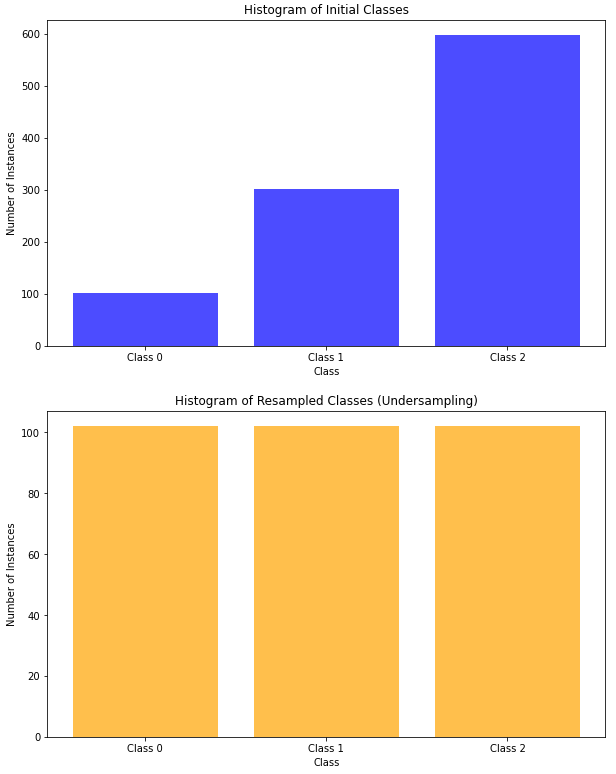
Comparing performances
Let’s create a Python example where we:
- Create an imbalanced dataset.
- Undersample and oversample it.
- Create the train and test sets for both the oversampled and undersampled datasets and fit them with a KNN classifier.
- Compare the accuracy of the undersampled and oversampled datasets.
import numpy as np
from sklearn.datasets import make_classification
from sklearn.model_selection import train_test_split
from sklearn.neighbors import KNeighborsClassifier
from imblearn.over_sampling import RandomOverSampler
from imblearn.under_sampling import RandomUnderSampler
from sklearn.metrics import accuracy_score

# Create an imbalanced dataset with 3 classes
X, y = make_classification(
    n_samples=1000,
    n_features=20,
    n_classes=3,
    n_clusters_per_class=1,
    weights=[0.1, 0.3, 0.6],  # Class imbalance
    random_state=42
)

# Split the original dataset into train and test sets
X_train, X_test, y_train, y_test = train_test_split(X, y, test_size=0.2, random_state=42)

# Apply oversampling using RandomOverSampler
oversampler = RandomOverSampler(sampling_strategy='auto', random_state=42)
X_train_oversampled, y_train_oversampled = oversampler.fit_resample(X_train, y_train)

# Apply undersampling using RandomUnderSampler
undersampler = RandomUnderSampler(sampling_strategy='auto', random_state=42)
X_train_undersampled, y_train_undersampled = undersampler.fit_resample(X_train, y_train)

# Fit KNN classifier on the original train set
knn_original = KNeighborsClassifier(n_neighbors=5)
knn_original.fit(X_train, y_train)

# Fit KNN classifier on the oversampled train set
knn_oversampled = KNeighborsClassifier(n_neighbors=5)
knn_oversampled.fit(X_train_oversampled, y_train_oversampled)

# Fit KNN classifier on the undersampled train set
knn_undersampled = KNeighborsClassifier(n_neighbors=5)
knn_undersampled.fit(X_train_undersampled, y_train_undersampled)

# Make predictions on train sets
y_train_pred_original = knn_original.predict(X_train)
y_train_pred_oversampled = knn_oversampled.predict(X_train_oversampled)
y_train_pred_undersampled = knn_undersampled.predict(X_train_undersampled)

# Make predictions on test sets
y_test_pred_original = knn_original.predict(X_test)
y_test_pred_oversampled = knn_oversampled.predict(X_test)
y_test_pred_undersampled = knn_undersampled.predict(X_test)

# Calculate and print accuracy for train sets
print("Accuracy on Original Train Set:", accuracy_score(y_train, y_train_pred_original))
print("Accuracy on Oversampled Train Set:", accuracy_score(y_train_oversampled, y_train_pred_oversampled))
print("Accuracy on Undersampled Train Set:", accuracy_score(y_train_undersampled, y_train_pred_undersampled))

# Calculate and print accuracy for test sets
print("\nAccuracy on Original Test Set:", accuracy_score(y_test, y_test_pred_original))
print("Accuracy on Oversampled Test Set:", accuracy_score(y_test, y_test_pred_oversampled))
print("Accuracy on Undersampled Test Set:", accuracy_score(y_test, y_test_pred_undersampled))
We obtain:
Accuracy on Original Train Set: 0.9125
Accuracy on Oversampled Train Set: 0.9514767932489452
Accuracy on Undersampled Train Set: 0.85

Accuracy on Original Test Set: 0.885
Accuracy on Oversampled Test Set: 0.79
Accuracy on Undersampled Test Set: 0.805
This comparison with the accuracy metrics shows the features of these methodologies because:
- The oversampling technique suggests that the KNN model is overfitting, and this is due to the oversampling itself.
- The undersampling technique suggests that the KNN model may be biased, and this is due to the undersampling itself.
- Fitting the model without resampling shows good performance of the model, because accuracy is misleading with imbalanced data.
So, in this case, a possible solution could be to use oversampling and tune the hyperparameters of the KNN to see if the overfitting can be avoided.
Ensembling
Another way to deal with imbalanced data is by using ensemble learning. In particular, Random Forest (RF) – which is an ensemble of multiple Decision Tree models – is a widely used ML model for its inherent ability to not favor the majority class.
Here’s why:
- Bootstrapped sampling. The RF models work with bootstrapped sampling, meaning that, during the training of the various DT models, the data selected are a random subset of the entire dataset, using replacement. This means that, on average, each decision tree is trained on only about two-thirds of the original data. As a result, some of the minority class instances are likely to be included in the subsets used to build decision trees. This randomness in sample selection helps to balance the influence of the majority and minority classes.
- Random feature selection. In addition to randomizing the data, Random Forest also randomizes the feature selection for each node of each tree. In other words, it selects a random subset of the features to consider when making a split. This feature randomness reduces the potential bias towards features that may predominantly represent the majority class.
- Error-correction mechanism. Random Forest employs an error-correction mechanism through its ensemble nature. If a decision tree in the ensemble makes errors in some minority class instances, other trees in the ensemble can compensate by making correct predictions for those instances. This ensemble-based error correction helps to mitigate the dominance of the majority class
Let’s consider the dataset we created before, and let’s use a Random Forest classifier to fit it:
import numpy as np
from sklearn.datasets import make_classification
from sklearn.model_selection import train_test_split
from sklearn.ensemble import RandomForestClassifier
from sklearn.metrics import accuracy_score

# Create an imbalanced dataset with 3 classes
X, y = make_classification(
    n_samples=1000,
    n_features=20,
    n_classes=3,
    n_clusters_per_class=1,
    weights=[0.1, 0.3, 0.6],  # Class imbalance
    random_state=42
)

# Split the dataset into train and test sets
X_train, X_test, y_train, y_test = train_test_split(X, y, test_size=0.2, random_state=42)

# Fit Random Forest classifier on the train set
rf_classifier = RandomForestClassifier(random_state=42)
rf_classifier.fit(X_train, y_train)

# Make predictions on train and test sets
y_train_pred = rf_classifier.predict(X_train)
y_test_pred = rf_classifier.predict(X_test)

# Calculate and print accuracy for the train set
train_accuracy = accuracy_score(y_train, y_train_pred)
print("Accuracy on Train Set:", train_accuracy)

# Calculate and print accuracy for the test set
test_accuracy = accuracy_score(y_test, y_test_pred)
print("Accuracy on Test Set:", test_accuracy)
And we obtain:
Accuracy on Train Set: 1.0
Accuracy on Test Set: 0.97
In this case, since we used the Random Forest, we didn’t need to resample the dataset. Anyway, the results suggest a possible overfitting of the model. This may be due to the Random Forest features itself, so further investigations will require hyperparameters tuning.
Anyway, in this case, using the RF model after hyperparameters tuning may be a good choice rather than undersampling or oversampling the dataseset and using the KNN.
Conclusions
In this article, we’ve discussed how to handle imbalanced data in Machine Learning.
In particular, there are situations where we expect the data to be imbalanced because we’re studying rare events.
Instead, in cases where the data must not be imbalanced, we’ve shown some methodologies on how to treat ML models like resampling and ensembling.